Nothing in this article is classified. Where I refer to Navy sonar and TMA data, I have cited official DoD sources in which the data has been publicly released. If you think I’ve made a mistake, you can email me at the address on my homepage.
I was lucky enough to deal with a lot of interesting problems during my time in the Navy. Today I’d like to share one that many Submariners encounter on a daily basis, and an unconventional way that I found to solve it.
Submarines employ sonar constantly to track targets, surface safely, and avoid detection. Sonar is a pretty famous technology, and you’ve probably heard that there are two principal types: active and passive. The following image is helpful.
An explanation of passive vs. active sonar from the BBC.1
Active sonar is similar to radar or lidar; a sound pulse is sent out from transducers on the ship, the sound bounces off objects, and then it returns after some time. The direction of the return gives the bearing (direction) to the target, and the elapsed time between ping and return gives the range (distance).
Because it gives both distance and direction, active sonar can determine the exact position of a target. Despite this, it has a few drawbacks. The most important is that it is detectable. A submarine’s chief advantage is stealth, and it’s difficult to be stealthy while pinging all the time. Since sound waves attenuate on the way to and from the target, a submarine using active sonar can be heard at twice the range of the farthest thing it can detect.
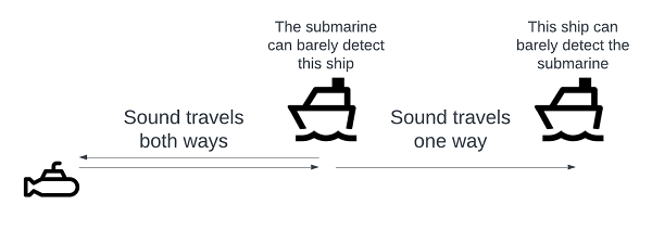
Original image.
Active sonar can also be environmentally unfriendly, and there are some places where naval vessels aren’t supposed to use active sonar, or have to reduce it, because of its effect on whales and other sea life.
Because of this, modern submarines typically use passive sonar. Passive sonar is a system more similar to directional listening. Submarines are equipped with hydrophones which listen to noises coming from different directions. The output of these hydrophones is processed to give precise bearing information on whatever noisy things happen to be nearby.
Passive sonar is stealthy and environmentally friendly, but it gives the operator less information than active sonar. Specifically, it only gives bearings. Since there’s no ping, the time between ping and return can’t be exploited to calculate the distance to the target.
I’ll be focusing this article on hull-mounted sonar arrays, but special types of array, like towed arrays, give even less information.2
Determining the target’s position from this list of bearings is called Target Motion Analysis, or TMA. In particular, this problem is known as bearings-only TMA, to differentiate it from other TMA situations where more information is available. Bearings-only TMA essentially boils down to determining range. Since bearing is known, an accurate range is enough to determine position. If position is known over time, it is easy to determine the target’s course and speed.
A bearings-only TMA visualization.3
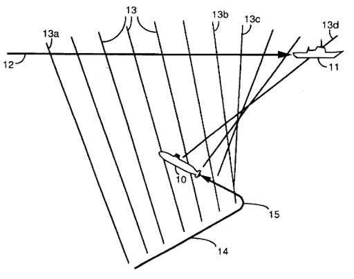
There is a simple method you might consider when facing this problem: using the sound’s volume (loudness). In air, sound volume mostly obeys an inverse-square law. It might make sense in air to sort sounds by volume and assume that the loudest sound comes from the closest object. This doesn’t work reliably underwater; different objects give off very different noise levels, and sound travels in exotic paths underwater, which can deaden or amplify noise.
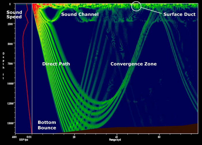
Examples of underwater sound propagation paths.4
While there are other ways to determine range, bearings-only TMA is often the best (or only) option.
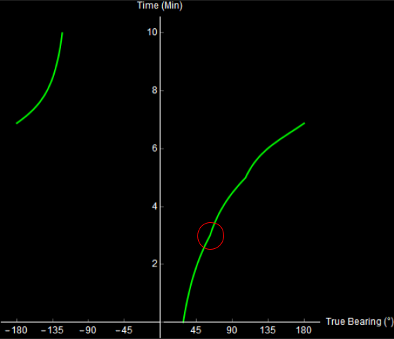
Consider the following situation. You are in a ship (or submarine) with hull-mounted sonar arrays. You are traveling North. On the right is what you see on your sonar display over 10 minutes.
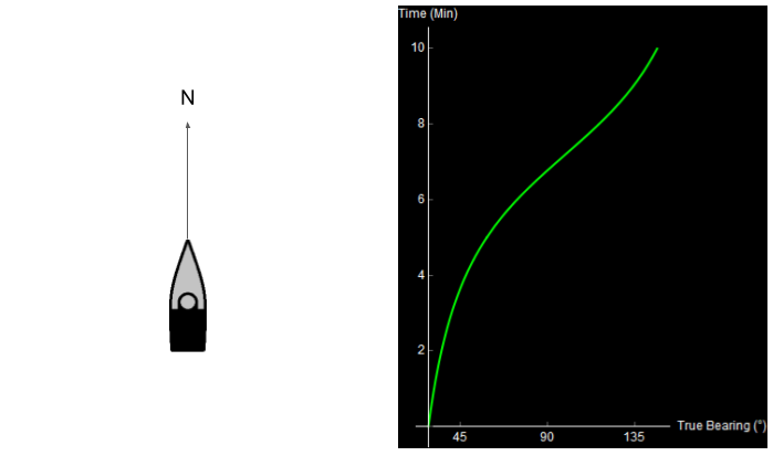
Original image.
On this sonar display, true bearing is shown on the x-axis (measured in degrees, clockwise from North). Time is shown on the y-axis, with the most recent bearing shown towards the top. What happened over these 10 minutes? Take a second to try and figure it out.
Qualitatively, you can already kind of tell what happened. Something noisy (a ship, maybe) started ahead and to the right of you, and then passed by your starboard side. I’ll cheat now and show you the data that I used to generate this image.
10 minutes of sonar data. The blue dot is your own ship, the red dot is the other ship. Watch the green crescent (bearing) change over time. Original image.
When we perform TMA, we use the data on the left to generate the picture on the right.
The key insight of TMA is what I call the two-range theorem.
If the target travels in a straight line at a constant speed, we can determine its entire path by determining two distances: the initial and final range (R1 and R2).
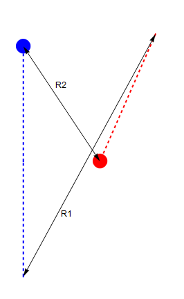
Original image.
As we vary our guesses for R1 and R2, we can use trigonometry to calculate the expected bearing trace over the 10-minute interval. If this lines up with the real trace, we likely have a good solution for the target’s range.
Varying guesses for R1 and R2. The red and green lines are the expected and observed bearing traces, respectively. They overlay when our choice of R1 and R2 is correct. Original image.
If we manually vary R1 and R2 like this, it’s difficult to consider all possible options. It’s quite possible that we might miss a good choice for R1 and R2 because we didn’t try it. Luckily, there’s a tool that allows us to simultaneously view every possible choice for the two ranges.5
We draw a contour plot with a range of possible values for R1 on the x-axis, and a range of values for R2 on the y-axis. Then we can color the area in with the error between the expected and observed bearing trace for each R1-R2 choice. The error is the area between the two curves.
\[\int_{t_0}^{t_1} \big\lVert\text{Observed BRG}(t)-\text{Predicted BRG}(t)\big\rVert\mathrm{d}t\]When we draw this contour plot here, it looks like this. Pink are areas of high error, green means low error. The small black dot is the actual value of R1 and R2.
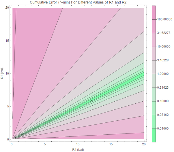
Original image.
Pick the greenest point on the contour plot, and you likely have a good solution for your target.
You could come up with a simple algorithm to “solve” bearings-only TMA like this:
Using gradient descent, this can all be automated. I’ll call this the conventional approach to TMA.
You might have noticed this, but there is a lot of green space on the contour plot above. In other words, there are many R1-R2 pairs that fit the data. This means that any TMA guess we make will be error-prone.
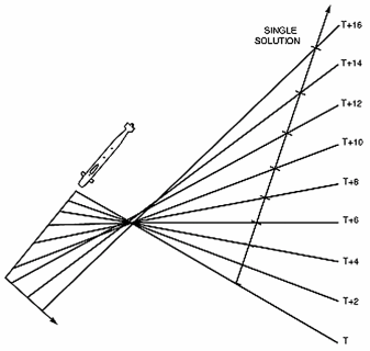
To see the problem, look at the following four paths. All of them are straight-line, constant-speed tracks, and all of them give the exact same bearing trace!
Original image.
Wagner, Mylander, and Sanders summarize this problem in Naval Operations Analysis as Theorem 11.4:
One cannot obtain target course, speed, or range from bearings only, no matter how numerous, when own track is linear.6
The problem here is fundamental, and no algorithm can save us. There is not enough data to make an accurate prediction about the target’s location. The only solution is to gather more meaningful data.
Watch what happens in the same situation, where we decide to turn our ship halfway through the simulation.
Original image.
Turning the ship allows us to discriminate between the otherwise identical traces. Similarly, our contour plot now contains only one small region of low error. The true solution lies in its center.
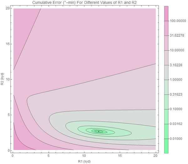
Original image.
The second problem will prove a little less tractable, and it’s to this issue that the rest of this project is devoted.
Consider the following situation. Your ship is traveling North for 5 minutes, and then turns to the Southeast for another 5 minutes. The resulting sonar trace looks like this. It’s worth mentioning that the bearing trace seen here is true bearing, measured from North, so it does not change when we turn.
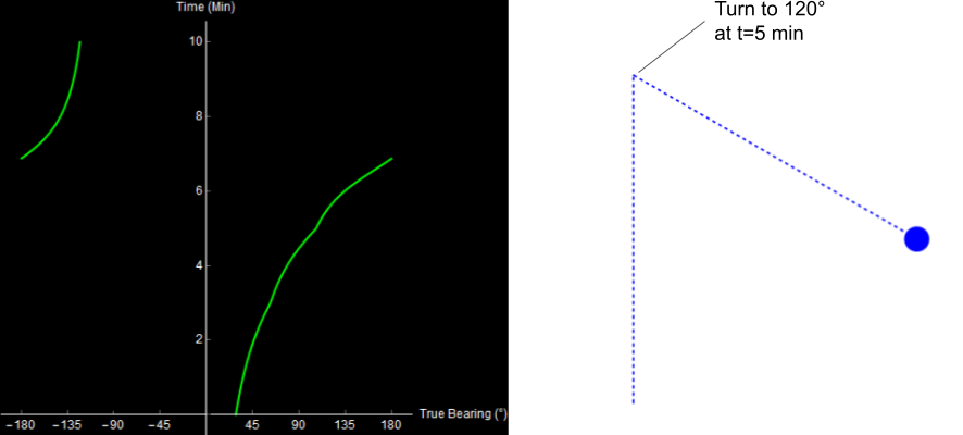
Original image.
Like before, I’ll let you try to figure out what is going on.
This time, we’ll use our newly-developed TMA algorithm to try and solve the problem.
Done.
Reading off the bearing trace, we get:
Initial: 30°
Final: -110° (or 250° for you nautical types).

Original image.
R1 = 9000 yards, R2 = 4800 yards
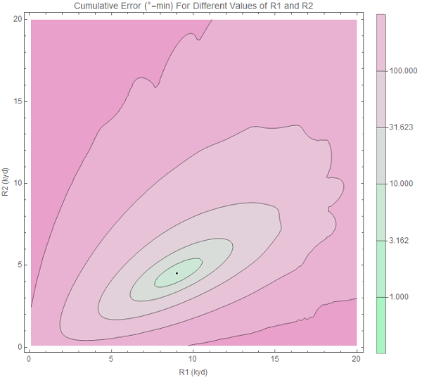
Original image.
When we plot the expected bearing trace, it looks pretty close to what we observed, and we might assume that the track on the right is correct.

Original image.
The problem is, that’s not what happened. The target actually turned 3 minutes into the simulation, and our calculated range is getting wronger by the minute!
Original image.
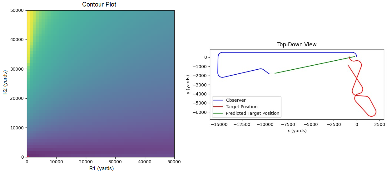
Why did our TMA algorithm fail us? Well, the 2-range theorem (and therefore our entire algorithm) relies on the assumption that the target traveled in a straight line. If the target turns or changes speed, our approach no longer works. This situation is far from unique. Here is a more complex example (it looks a little different because I simulated it in Python, not Mathematica).
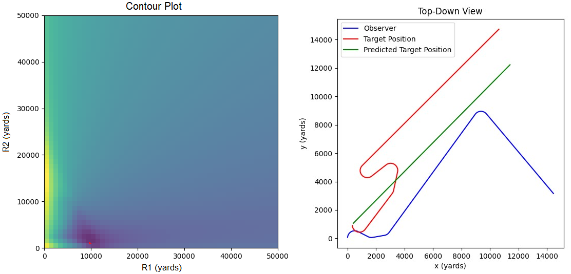
The red dot on the left is the point of minimum error. This corresponds to the green line on the right. The red line is the target’s actual track. Original image.
Sometimes, the solutions proposed by this TMA method are completely wrong.
Original image.
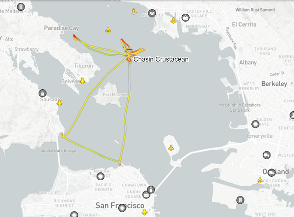
This is a serious problem! The accepted algorithm for TMA is based on an asymmetrical assumption: we must turn, but the target cannot. Turning targets are incredibly common, though. See this recent AIS track of a fishing vessel in San Francisco bay (Via MarineTraffic).
In a military context, zig-zagging has been a well-known defense against submarine attack for over 100 years!
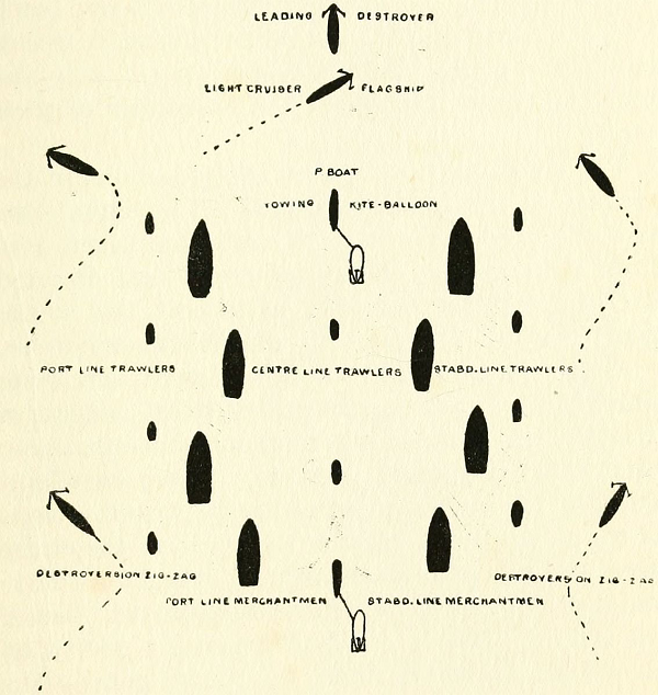
A 1920 illustration of a convoy employing anti-submarine measures. Notice the zig-zagging destroyers on the outer edge.7
The Navy has known about this problem since the introduction of straight-line TMA methods. To solve it, submarines employ 7 or 8 people at all times to look for indications of a target turning or changing speed. When this “zig” occurs, TMA models are reset and the operators start over.
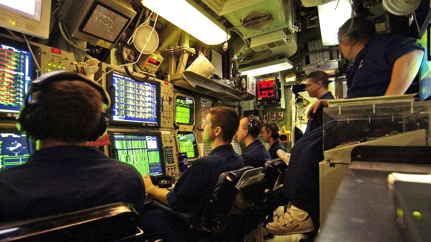
A submarine sonar shack, manned 24/7 while at sea. Among other tasks, these Sailors look for zigs.8
This means that every little indication of a turn has to be identified, or else the TMA algorithms will spit out a bad (and possibly worsening) solution. In practice, it’s difficult to get this right. Here is the zig from earlier, can you see the small corner? Would you reliably notice it?
Original image.
The approach does not scale. Imagine the same small team trying to analyze this contact picture.
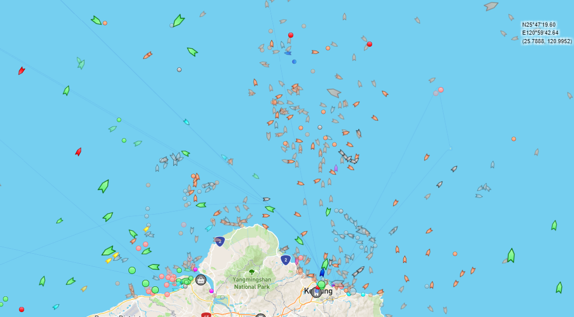
“Trawler Hell” North of Taiwan (via MarineTraffic).
Even in smaller, more controllable situations, TMA errors occur. This photo of a periscope was taken from a ferry in the UK, after a British submarine came dangerously close to collision. A TMA error proved responsible; the submarine’s crew incorrectly calculated the ferry’s speed.9
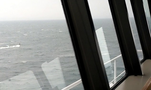
A bad day at work.9
Smaller non-military submarines and autonomous Unmanned Undersea Vehicles (UUVs) also cannot employ the Navy solution to problem 2, because they don’t have the manpower aboard to support zig detection.
For these reasons, we need a fully automatic solution for TMA.
Intuitively, I felt like a solution without the straight-line model was possible. This seemed like an overdetermined system to me: there are many bearing measurements, and comparatively few unknowns (turns).
Many bearings, few turns.10
This problem rolled around in my head for a few years before I took a certification course in machine learning. In the course, I saw how Recurrent Neural Networks (RNNs) could be applied to time-series data, and thought that this might be the TMA tool I was looking for.
A RNN is a type of neural network in which output from some nodes is reintroduced as input to the same nodes. RNNs are good at forecasting time series, because they can handle variable length input, and retain context over many time steps.
My basic idea was to use a RNN to translate bearing time steps to range time steps. As the simulation continued, the model would hopefully pick up context about its situation through the recurrent link, and produce better and better predictions.
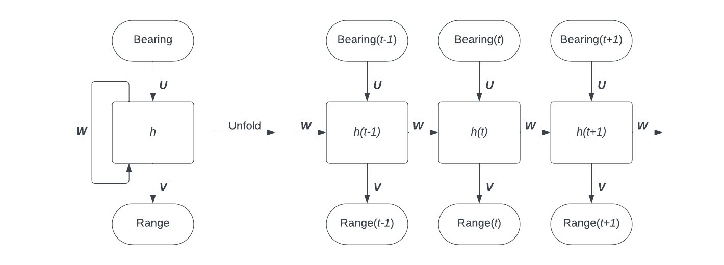
A simple model of a TMA RNN. The network is unfolded on the right to show how data flows between time steps. U, V, and W are combinations of weights and biases which are applied to process input, process output, and retain context respectively, while h is the system’s hidden state, a vector which stores information up to the current time step. Original image.
In reality, I chose a more complex model. Bearing alone isn’t enough, I needed the friendly ship’s speed as well. I split bearing up into relative bearing and true bearing-rate. This way, I could preserve all necessary information while also making the problem rotationally invariant; it shouldn’t matter which way North is.
Simple RNNs suffer from an issue called the vanishing gradient problem, which limits their ability to retain context over long periods. This could make it difficult to process hundreds of bearings. To fix this, I employed a type of RNN called a Long Short-Term Memory cell, or LSTM cell. An LSTM cell chooses what information to remember and what to forget, with the goal of only retaining important context.

An illustration of an LSTM cell by Guillaume Chevalier. CC-BY-SA, no changes made.
I used two LSTM cells, the first with 32 output units and the second with 16. I was inspired by the following piece of neural network “lore”, from Stephen Wolfram:
One can often get away with a smaller network if there’s a “squeeze” in the middle that forces everything to go through a smaller intermediate number of neurons.11
Here is a diagram of the network design I actually used. I’ll explain the dropout layers when I talk about overfitting.
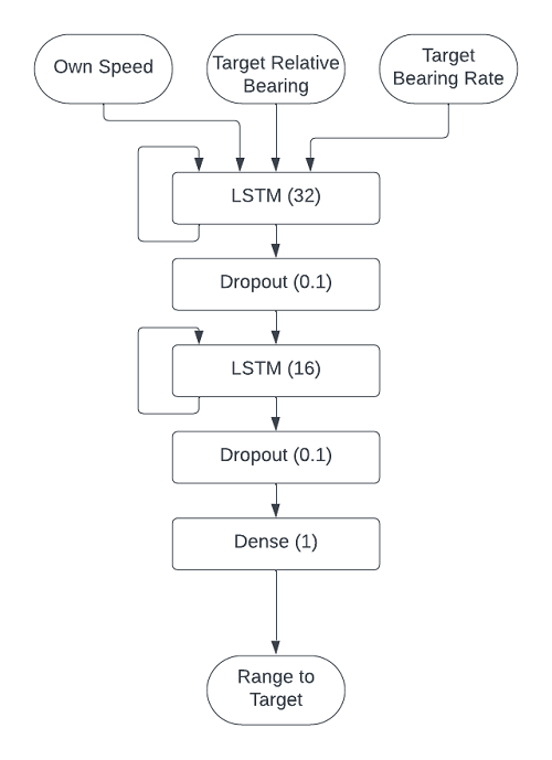
Original image.
I implemented the model in Python, with Tensorflow and Keras, on a Windows desktop computer. Since Tensorflow removed support for GPUs in native Windows, I used WSL2 to train my network using my graphics card.
For my training set, I wrote a script to simulate two ships driving and turning at random. I ran 50,000 simulations, each one 50 minutes long with bearings taken every 10 seconds. The ships drove at random speeds between 5 and 25 knots, and started in a 2000 by 2000 yard box. Both ships turned to random courses at random intervals, every 1000 seconds on average. I split my data into training (80%) and validation (20%) sets. I used a Mean Squared Error loss function, since I wanted to punish large errors more than small errors.
I did a preliminary training run where I varied learning rate over several orders of magnitude. This helped me find an appropriate rate: slow enough to allow stable training but fast enough to save time.
I employed a 4-prong defense against overfitting.
I also varied batch size during training, which caused the spikes on the loss graph below. Honestly, I don’t know if it was helpful, but it allowed longer training runs before early stopping terminated training.
My first training run took about an hour, and looked like this.
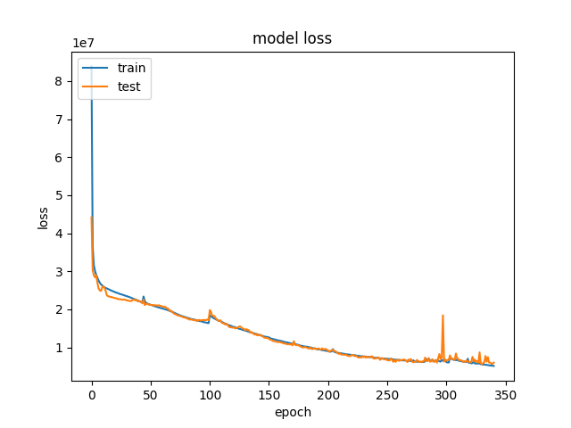
Original image.
After I stopped seeing results, I lowered the learning rate by two orders of magnitude, and that helped me cut the loss in half on my second training run.
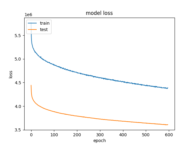
Original image.
Note that the validation loss is consistently lower than the training loss. In other words, the model is performing better on the validation set than the training set. This surprised me. At first I thought that this was because training loss is calculated during training, and validation loss is calculated afterwards. That hypothesis doesn’t really fit the data, though, since the gap is persistent over multiple epochs. Instead, I think this is because of dropout: the model is less powerful during training because 10% of its connections have been pruned, while all of its connections are active during validation.
After training, I tested the model on 5000 new simulations not in the training or validation sets. I wrote a script to automatically apply the conventional TMA algorithm, and compared it with the ranges calculated by the machine learning model. To evaluate accuracy, I calculated the Mean Squared Error (MSE) and Mean Absolute Error (MAE) for both methods.
| Conventional TMA | Machine Learning Model | |
| Mean Squared Error | 1.114 × 10⁸ yards2 | 3.838 × 10⁶ yards2 |
| Mean Absolute Error | 7139 yards | 1265 yards |
For MSE, the machine learning model is 2 orders of magnitude better than the conventional method. On average, the conventional method is off by over 7000 yards, while the machine learning model is within a comfy 1500 yards.
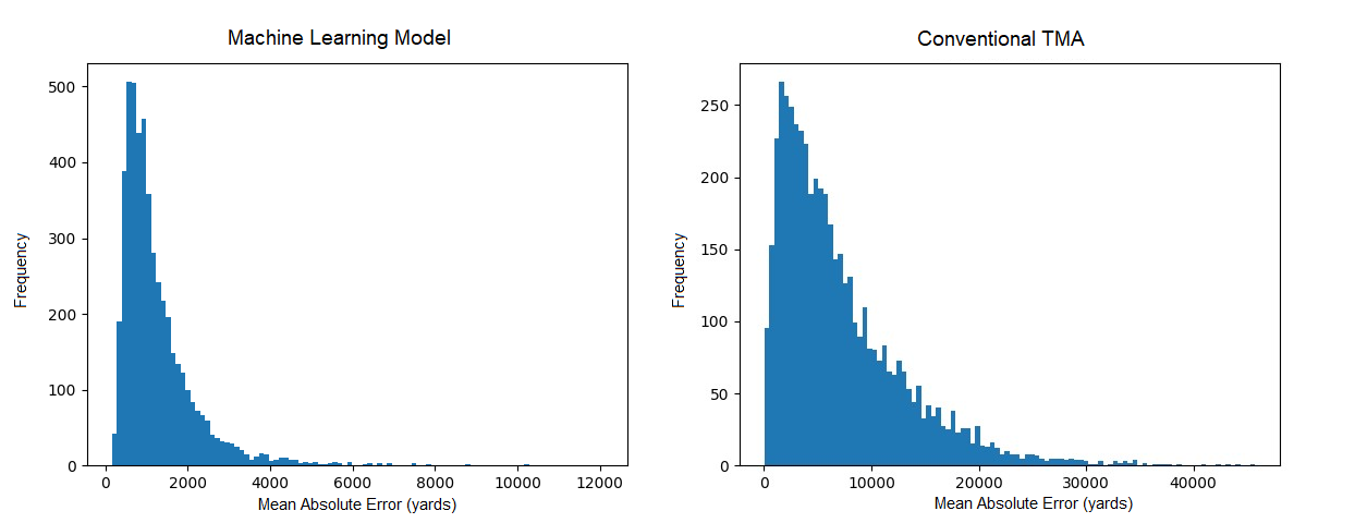
Histograms of the model’s Mean Absolute Error on the 5000-simulation test set. If these look too similar, check the scale on the x-axis! Original image.
The histograms above show that the machine learning approach virtually guarantees MAE within 4000 yards, where conventional TMA is often off by over 15000!
To someone with Naval experience, this difference in performance is huge and obvious, but for the rest of us, I will show a few simulation examples to demonstrate what a MAE of 1265 yards actually looks like.
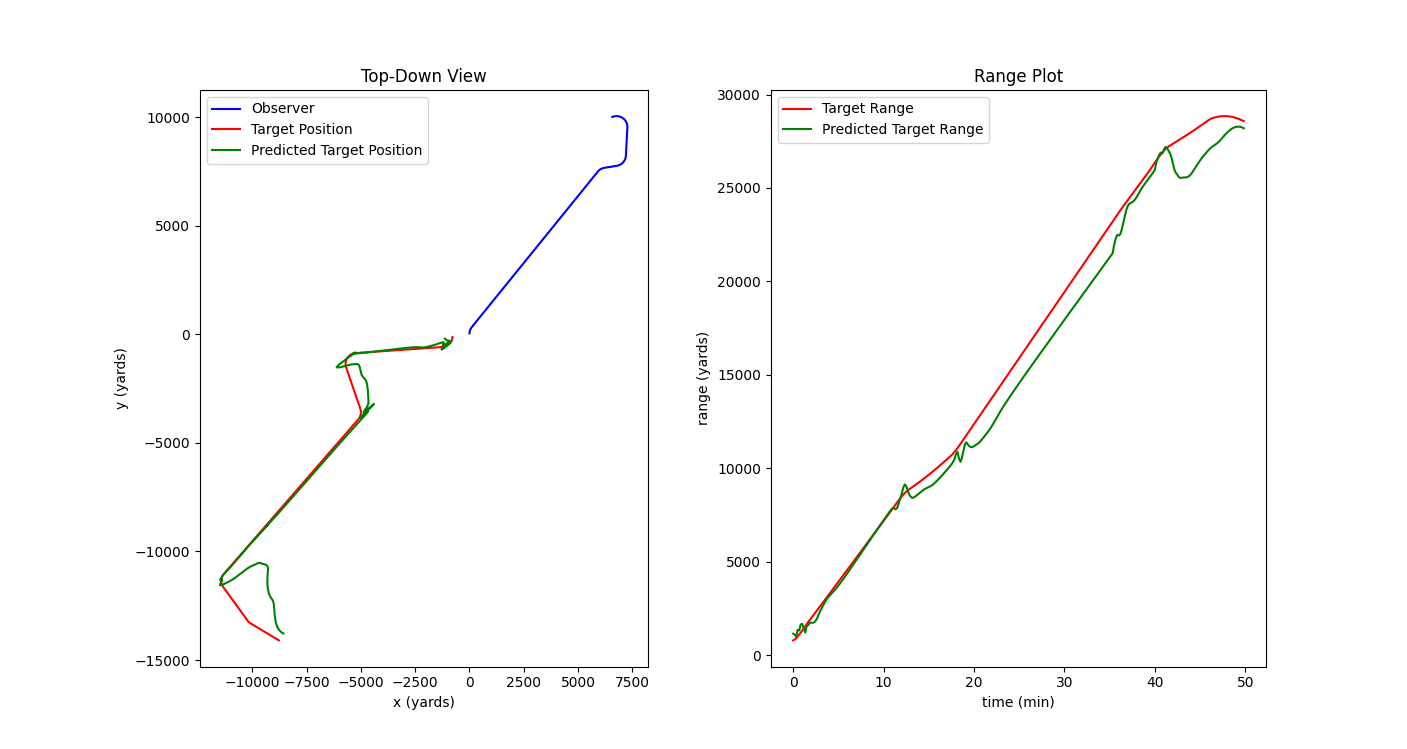
Better than average performance. Range accuracy is almost perfect throughout the simulation. On the left, the green line (predicted target position) overlays almost perfectly with the red line (actual target position). MAE: 873 yards. Original image.
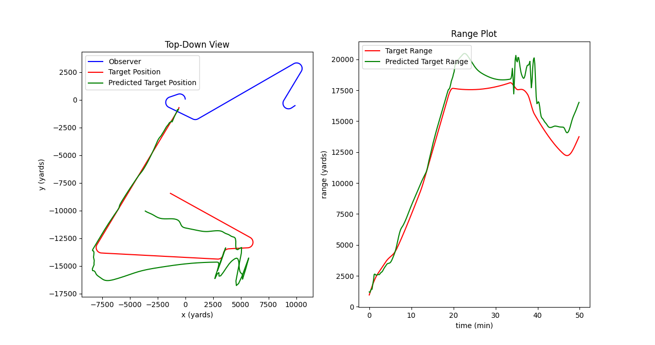
About average performance. The model has difficulty determining target range immediately following the target’s first turn, but eventually figures out the target’s approximate motion path. This is an accurate enough tactical picture for most situations. MAE: 1153 yards. Original image.
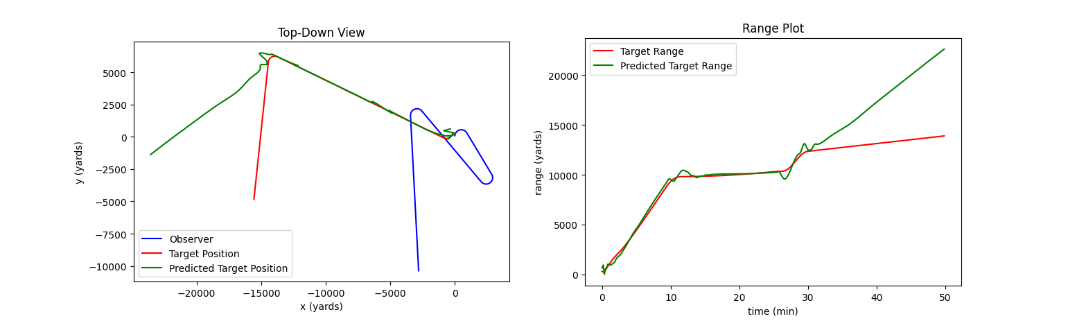
Worse than average performance. The model calculates range correctly until the target turns onto a near-zero bearing-rate path. In fairness, this is a very difficult situation, and I have seen people make similar mistakes. MAE: 1814 yards. Original image.
The model that I trained is essentially a proof of concept, and this project is not ready for any real use yet. It would be prudent to explore a few related topics first.
Better Evaluation. The comparison above is not exactly fair, because conventional TMA tools were not designed to be fully autonomous; it would be better to evaluate the model against a skilled human. It would be cool to evaluate or train this model on real sonar traces, rather than simulation data. I have also thought about introducing bearing error into the training and evaluation data, or limiting precision. All of these would help evaluate the model under more accurate conditions.
A Better Model. The model can only deal with a small number of inputs and conditions right now. To be useful in real life, it would need to be able to interpret intermittent contact with targets, and targets with varying speed. It would also be useful to specify speed constraints for the model to limit its output options (if, for example, the target had a known maximum speed). Finally, a custom loss function (rather than MSE) could probably improve the model’s accuracy by penalizing it when it created unrealistic tracks (for example, range jumps between time steps).
Non-Machine-Learning Additions. Probably the best way to improve the model’s performance would be to apply non-ML methods to its input or output. For example, smoothing the output would prevent the oscillations which often occur after the target turns. We could also use a hybrid approach to get the best elements from conventional TMA and machine learning: for example, using a ML model to detect turns and conventional TMA to fill in the blanks between them.
Kaouri, Katerina. Left-right ambiguity resolution of a towed array sonar. (2000). 7. ↩
Nguyen, Steiner, & Scales. Optimized deterministic bearings only target motion analysis technique. (1998). U.S. Patent No. 5,732,043. ↩
US Navy. Environmental Impact Statement/Overseas Environmental Impact Statement, Atlantic Fleet Training and Testing. (2017) 16. ↩
Blaylog and Ganesh. System and method for target motion analysis with intelligent parameter evaluation plot. (2003). U.S. Patent No. 7,020,046 B1. ↩
Wagner, Mylander, & Sanders. Naval Operations Analysis. (1999) Naval Institute Press. 259. ↩
Domville-Fife. Submarine Warfare of To-Day. (1920). Seely, Service & Co. Ltd. 119. ↩
US Navy via Amick. How Submarine Sonarmen Tirelessly Hunt For Enemies They Can’t Even See. (2020). The Drive. ↩
Ng. British nuclear submarine in ‘near miss’ with packed ferry after ship sees periscope. (2020). The Independent. ↩ ↩2
Milazzo. Performing Automatic Target Motion Analysis. (2011). ↩
Wolfram. What is ChatGPT Doing… And Why Does it Work? (2023). Wolfram Media. ↩
Srivastava, Nitish, et al. Dropout: a simple way to prevent neural networks from overfitting. (2014). The journal of machine learning research: 15.1. 1929-1958. ↩