Imagine a cannon, firing a shell into the air. What path will the shell follow? How far will it travel? How long will it remain airborne? Below is woodcut by Walther Hermann Ryff, a 16th century mathematician, examining this question. At the time, most theorists thought that cannonballs traveled in straight-line segments and circular arcs, stitched together.
Nowadays, we know better. There is a simple, Newtonian treatment of projectile motion which we learn in high school or early college level physics. The problem has clear analytical solutions which you’ll probably recognize: projectiles travel in parabolas, there is a closed-form range and hang time equation, which you may know, etc. It reminds me of some other early physics topics, which contain a simplifying assumption which makes the problem manageable.
| Problem | Simplifying Assumption |
|---|---|
| Motion of a pendulum | Small-angle approximation |
| Motion of a block sliding down a plane | Neglecting friction |
| Mass on a pulley | Neglecting friction |
In this case, the main simplifying assumption is to neglect air resistance. This makes the equation of motion simple and linear. Gravity is the only acceleration affecting the projectile. Therefore, the horizontal and vertical accelerations \(a_x\) and \(a_y\) are given by:
\[\begin{align} a_x &= 0\\ a_y &= -g\\ \end{align}\]Where \(g\) is the acceleration of gravity, 9.81m/s2. The initial horizontal and vertical velocities \(v_x\) and \(v_y\) are given by:
\[\begin{align} v_x &= v_0\cos\theta\\ v_y &= v_0\sin\theta\\ \end{align}\]Where \(v_0\) is the launch speed and \(\theta\) is the launch angle. If we assume that the mass starts at the location \((0,0)\), then this reduces to the following initial value problem:
\[\begin{align} \frac{\mathrm{d}}{\mathrm{d}t}\left(x\right) &=v_x, &x(0) &= 0\\ \frac{\mathrm{d}}{\mathrm{d}t}\left(y\right) &=v_y, &y(0) &= 0\\ \frac{\mathrm{d}}{\mathrm{d}t}\left(v_x\right) &=0, &v_x(0) &= v_0\cos\theta\\ \frac{\mathrm{d}}{\mathrm{d}t}\left(v_y\right) &=-g, & v_y(0) &= v_0\sin\theta\\ \end{align}\]Integrate this, and you get a general equation for the projectile’s speed and velocity.
\[\begin{align} x(t) &= v_0t\cos\theta\\ y(t) &= v_0t\sin\theta-\frac12gt^2\\ v_x(t) &= v_0\cos\theta\\ v_y(t) &= v_0\sin\theta - gt\\ \end{align}\]You can plot this parametrically, and sure enough, it is a neat parabola.
If you play with the launch angle (\(a\) here, since \(\theta\) is used to plot polar graphs) you can see that an angle of 45° produces the maximum range. If you want to prove this, you can derive the range equation.
We know the target will hit the ground when \(y=0\). Since we have an expression for \(y\), we can solve this explicitly.
\[\begin{align} y(t) =0 &= v_0t\sin\theta-\frac12gt^2\\ &= t\left(v_0\sin\theta - \frac12gt\right)\\ \Rightarrow 0 &=t\left(t-\frac{2v_0\sin\theta}g\right)\\ \Rightarrow t &= 0 \text{ or } \frac{2v_0\sin\theta}g \end{align}\]So \(y=0\) at launch time (when \(t=0\)) and at the end of the trajectory (when \(t=\frac{2v_0\sin\theta}g\)).
Substituting this value of \(t\) into our equation for \(x\), and using the double-angle sine identity, we get:
\[\begin{align} x(t) &= v_0t\cos\theta\\ x\left(\frac{2v_0\sin\theta}g\right) &=\frac{2v_0^2\sin\theta\cos\theta}{g}\\ &=\frac{v_0^2\sin(2\theta)}{g} \end{align}\]This formula tells us a couple interesting things. First of all, the range of the projectile is indeed maximized when \(\theta = 45^\circ\), because \(\sin(2\theta)=1\), its maximum value. It also tells us that there are always two angles which give us the same range. Try varying the launch angle in the plot below.
The second insight is particularly useful, and was used in World War II to great effect. It allowed a tactic called “time on target,” where artillery guns would first fire a high shot, and then a low shot after a specified time. Since they would travel the same range, but in different times, both shells would strike the target simultaneously.
If the cannon is able to vary the launch speed, as well as the launch angle, there can be a greater number of simultaneous shots, limited only by the gun’s ability to reload. See the below image from the wikimedia commons.

This concept is now known as multiple round simultaneous impact, or MRSI. The best modern guns can fire up to six MRSI rounds (link to brochure) at close range.
So why write about this at all? We already have it figured out. I was interested in this topic, because everything I’ve learned about projectile motion has the simplifying assumption that I mentioned early in the article: no air resistance. The problem is, air resistance is significant! Shells are heavy, but not too heavy, and at their supersonic speeds, air resistance is a huge, nonlinear factor, which makes the above equations unrealistic for most cases—definitely not realistic enough to base artillery fire on. So, I wanted to use some simulation to look at how air resistance affects projectile motion at fast speed.
Air resistance is a messy topic. There are two main transitions which affect its magnitude.
The first transition happens when air flow around the object moves from laminar to turbulent. The transition between flow types depends on the Reynolds number, a dimensionless constant. We can calculate it like this:
\[\mathrm{Re}=\frac{uL}{\nu}\]Where \(u\) is the speed through the fluid, \(L\) is the characteristic length (for us, the shell caliber), and \(\nu\) is the kinematic viscosity of the fluid.
To figure out the approximate Reynolds numbers we’re working with, we can do some Fermi estimation. The kinematic viscosity of air is around 1.5 x 10⁻⁵ m2/s (so call it 10-5). A typical howitzer shell is around 150 mm caliber (0.1 m) and travels around 684 m/s (call it 1000). Doing the math:
\[\mathrm{Re}=\frac{1000\text{ m/s}\times0.1\text{ m}}{1\times10^{-5}\text{ m}^2\text{/s}}=10^{7}\]At high Reynolds numbers like this, fluid flow will be turbulent (even if we’re off by an order of magnitude or two). This means that the shell will be subject to Newtonian drag. In other words, the drag will be proportional to the square of the object’s velocity.
\[F_d=\frac12\rho v^2c_dA\]Where \(F_d\) is the force of drag, \(\rho\) is the fluid density, \(c_d\) is the drag coefficient, and \(A\) is the cross-sectional area of the shell.
All of these values are easy to find, except the drag coefficient. This is where I had to focus on a particular test case, and where we run into the second transition.
Non-rocket-powered artillery is typically split into three categories: cannons, which fire shells at low angles, mortars, which fire shells at high angles, and howitzers, which fire shells over a range of angles in between the other two. Since I was interested in choosing a variety of launch angles, I chose a howitzer.
There are a few to choose from, but the long-time favorite of the US and several other countries is the M198. This is a great choice for analysis because it has been used over several decades, and there is a lot of good data available (more on this later).
A common shell fired by the M198 howitzer is the M107 projectile. Even though it’s since been superseded by better projectiles, it’s still seen a fair amount of use, especially in training and testing. Here’s a photo from page 3-77 of Army TM 43-0001-28.
Here is some data which will be important:
| M198 Howitzer | M107 Shell |
|---|---|
| Angle Range: -5° to +72° | Diameter: 154.71 mm |
| Muzzle Velocity: 684 m/s | Mass: 43.2 kg |
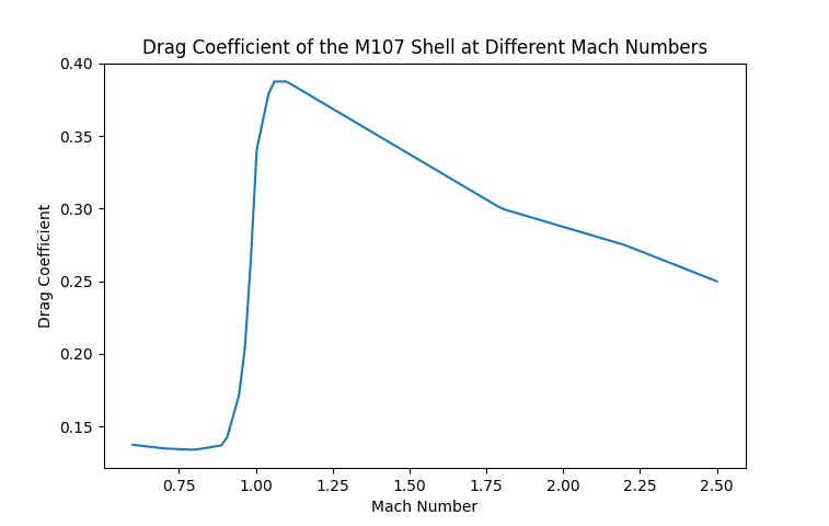
There’s some data out there about the aerodynamics of the M107 shell, including this paper by Garner et al., which directs the reader to a detailed analysis of the similarly-shaped M101 projectile by MacAllister and Krial. If you go to figure 7 of the paper, you can find this diagram:
In case it is too tough to read (the scan quality is terrible), the x-axis is the Mach number, the ratio of projectile speed to the speed of sound, and the y-axis is the zero-yaw drag coefficient \(c_{d0}\), which is equal to \(c_d\) if the projectile is parallel to its flight path.
You can see that the graph is really nonlinear; this is the second transition. At speeds below the speed of sound, the projectile has a mostly-constant \(c_{d0}\) of around 0.13. In the transonic range (near mach 1) the \(c_{d0}\) rises sharply to almost 0.4, before lowering again at higher Mach numbers. This is due to wave drag. At Mach numbers near 1, the compression effects of air become significant, and shockwaves form. Shockwaves cause large amounts of drag due to the sudden change in pressure along the wave front. The drag coefficient is actually greater at Mach 1 than at higher speed, since at Mach 1 the shock wave is perfectly normal (perpendicular) to the flight path, and exerts the most slowing pressure. Look at the shapes of the following shock waves at different Mach numbers to see what I’m talking about (source: James and Carros, Experimental Investigation of the Zero-Lift Drag of a Fin-Stabilized Body of Fineness Ratio 10 at Mach Numbers Between 0.6 and 10).
To use this data in calculation, I used scipy’s linear interpolation function, and selected some points from the graph to plot. Here’s what my drag coefficient curve looked like.
For the other components of the drag equation, I could just use standard values of air pressure, temperature, sound speed, etc. But since I’m already numerically simulating, there’s no reason to make these types of simplifications.
In a perfect, frictionless world, we can find the maximum expected height of the shell by doing a potential/kinetic energy balance. If the shell is launched perfectly upward, all its kinetic energy at launch time will be converted to potential energy at its apex.
\[\begin{align} KE_{\text{launch}} &= PE_{\text{apex}}\\ \frac12mv^2_{\text{launch}}&=mgh_{\text{apex}} \end{align}\]Mass cancels, and we can rearrange to find apex height.
\[\begin{align} h_{\text{apex}}&=\frac{v^2_\text{launch}}{2g}\\ &=\frac{(684\text{ ms}^{-1})^2}{2\times9.81\text{ ms}^{-2}}\\ &=23,846\text{ m} \end{align}\]So the maximum possible height that the M198 could launch the shell is nearly 24 km in the air, in the lower region of the stratosphere. At this height, the atmospheric pressure is about 1.6% of the pressure at sea level. This will affect drag a lot! Because of this, I decided it was necessary to factor in atmospheric properties at different heights.
What properties, exactly? Atmospheric density will be necessary, since it factors directly into the drag equation, but the speed of sound is also important, since it determines the Mach number. We can determine these from atmospheric pressure and temperature.
Atmospheric pressure and temperature vary with height in a strange way, since the atmosphere is unevenly heated by sunlight. Here’s a graph made by NASA in the sixties:
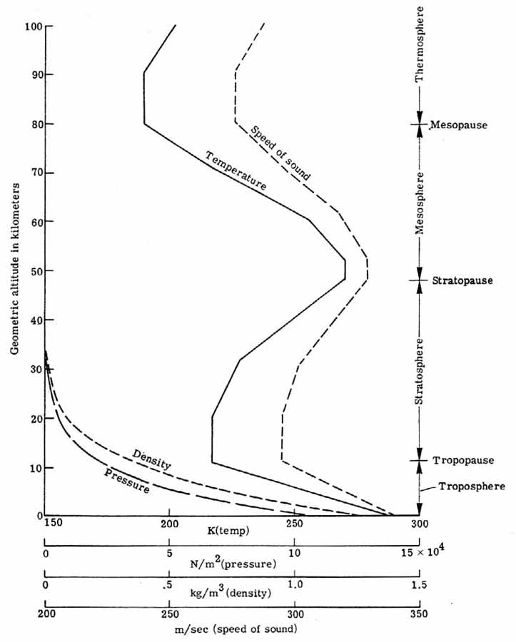
There is a formula for atmospheric pressure within the troposphere (the lowest portion of the atmosphere), but this relies on atmospheric temperature lowering linearly as height increases. From the graph above, we can see that this isn’t true, even at the relatively low heights to which our projectiles will travel. Instead, I used values from this table for both temperature and pressure, and interpolated. I converted the temperatures to Kelvin, and the pressures to Pascals, to keep everything in SI units.
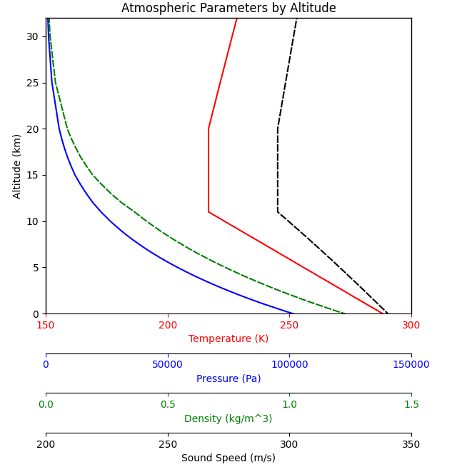
There are accurate formulae to calculate sound speed and density from this data.
\[\begin{align} c &=\sqrt{\gamma\times\frac{p}{\rho}}\\ \rho &=\frac{pM}{RT} \end{align}\]Where \(c\) is the speed of sound, \(\gamma\) is the heat capacity ratio (around 1.4 for dry air), \(p\) is the pressure, \(\rho\) is the density, \(M\) is the molar mass of dry air (around 0.029 kg/mol), \(R\) is the gas constant (8.32 J/K mol), and \(T\) is the absolute temperature.
Here’s my version of NASA’s graph, up to 32 km, which looks pretty much the same.
To see how the drag force will respond to altitude and speed, we can substitute these values into the drag equation, and draw a 2-d contour plot.
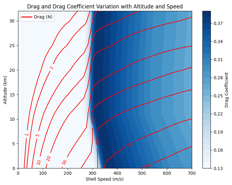
You can really see the “sound barrier” here, where drag sharply increases with shell speed. We’ll come back to this diagram later, when analyzing each shell’s trajectory.
Now that we have a reasonable model built, let’s analyze some actual shell paths!
The differential equations from the first section have an extra drag term inserted now, which is parallel to the particle’s velocity, and in the opposite direction.
\[\begin{align} \frac{\mathrm{d}}{\mathrm{d}t}\left(x\right) &=v_x, &x(0) &= 0\\ \frac{\mathrm{d}}{\mathrm{d}t}\left(y\right) &=v_y, &y(0) &= 0\\ \frac{\mathrm{d}}{\mathrm{d}t}\left(v_x\right) &=-F_{d}\frac{v_x}{\sqrt{v_x^2+v_y^2}}, &v_x(0) &= v_0\cos\theta\\ \frac{\mathrm{d}}{\mathrm{d}t}\left(v_y\right) &=-g-F_{d}\frac{v_y}{\sqrt{v_x^2+v_y^2}}, & v_y(0) &= v_0\sin\theta\\ \end{align}\]Where \(F_d\) is the force of drag, given by the drag equation from earlier.
\[F_d=\frac12\rho v^2c_dA\]This differential equation is not analytically solvable (especially considering how drag depends on speed and altitude), but we can solve it numerically, which I did with scipy’s solve_ivp function. Here’s an example of how the trajectories look, compared to the ideal, frictionless parabolas.
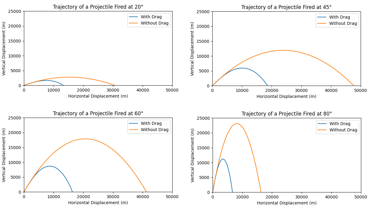
Clearly, drag makes a huge difference here. To see how big a difference, we can plot the ranges with drag and without drag over the entire span of launch angles.
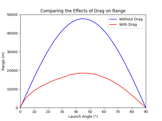
We can learn a few things from this angle/range plot. On the left edge of the graph, at low launch angles, the expected ranges with and without drag are much closer than on the right. This makes sense, since a shell fired at a low angle travels a shorter distance in the air, so less energy is lost to drag. It’s also worth noting that the maximum range estimate given by the drag model is much closer to the real maximum range of the M198 howitzer, which is listed publicly as 18,100 m when firing the M107 projectile.
What this graph doesn’t tell us, though, is what happens to the shells as they fly through the air: their speed, where they lose the most energy, etc. For this, I decided to display some trajectories on the speed/altitude graph.
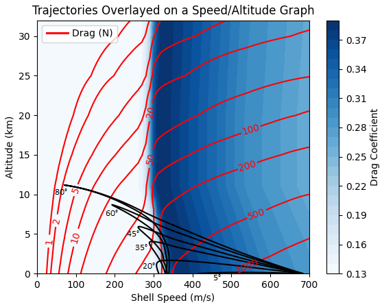
One of the really interesting things to gain from this graph is the final speed of each projectile. The 5° projectile loses very little energy, because it travels a very short distance, but the 20° projectile has the lowest final speed, which means that it has lost the most energy to air resistance. It is a sort of compromise: it has traveled far enough to lose significant energy to air resistance, but not high enough to escape the high-drag regions.
It’s also interesting to note that all projectiles spend a fair amount of their flight time subsonic. Even the 80° projectile, which spends a good portion of its flight time in a low-drag region, is unable to break the sound barrier on its descent. This has implications for artillery defense: it’s fairly certain that an incoming shell will arrive just under the speed of sound, no matter what the launch angle is.
Now that we have much better estimations of speed and range over a flight path, we can reexamine the time-on-target idea. When I started writing this, I was hoping that it would allow three or more shots to hit the same target without varying the initial shell speed. This is possible for certain niche values of speed, mass, and range. Here’s an example:
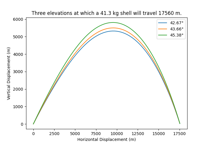
This isn’t practical, though. The shells are launched too close together, and the hang times are too similar. For most ranges and launch speeds, it doesn’t work.
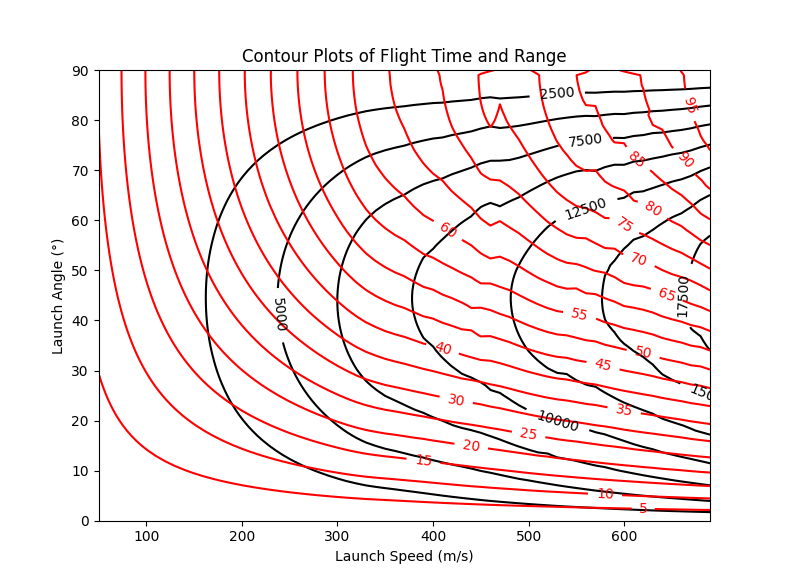
We can use the simulation data to generate a practical graph for MRSI when varying launch speeds, though. See the following contour plot. Red lines are flight time contours, and black lines are range contours.
The M198 can reload up to 4 times in one minute (once every 15 seconds). Suppose you wanted to hit a target 5000 yards away. You can highlight speed/angle combinations which would hit the desired target, and shoot all of them, as long as they are 15 seconds or greater apart.
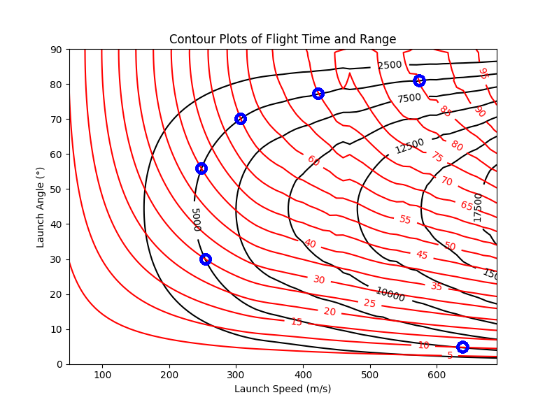
Following this plan, we could hit the target with 6 simultaneous shots!
| Time | Angle | Speed |
|---|---|---|
| +0 s | 81° | 576 m/s |
| +15 s | 77° | 420 m/s |
| +30 s | 70° | 306 m/s |
| +45 s | 56° | 248 m/s |
| +60 s | 30° | 253 m/s |
| +75 s | 5° | 621 m/s |
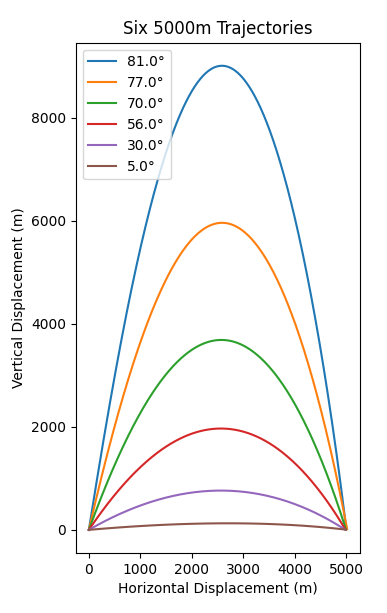
All shots would arrive at time +85s. Here’s a plot.
To see how accurate this all was, I tried to find a firing table, but the Army website wouldn’t let me in. Probably for the best…
Based on the maximum range, I’m satisfied with the quality of my simulation. There are a lot of other places we could go from here. It would be cool to incorporate orbital effects or vary the temperature and pressure. We could also shoot between different altitudes, or through a more viscous fluid! For now, though, I think this article has gone on long enough.