In 2020, I read Lample and Charton’s Deep Learning for Symbolic Mathematics. I had graduated with a math degree less than two years before, and I thought it would be cool to apply neural networks to math. One candidate was the search for Lyapunov functions, which were crucial to my undergraduate research. Finding Lyapunov functions is like finding integrals. The two problems share a tantalizing property: solutions are easy to verify, but hard to compute. I tried to reproduce some of Lample and Charton’s work on my own, but I wasn’t a great programmer. I was also distracted with my day job—I spent 260 days at sea in 2020.
A few weeks ago I decided to give it another shot. I’ve changed a lot since 2020, and now programming is my day job. I experienced success this time, but I chose to write here about the parts I found hard, and what surprised me about this project.
The machine learning aspect of this project wasn’t complex. In fact, my goal was less ambitious than the authors of the paper. Instead of creating a model which could perform integration, I wanted to create a model which could determine if a function was integrable. I would generate a bunch of random functions, use a computer algebra system (CAS) to try and integrate them, record which ones were integrable and which weren’t, and train a text classifier to determine which was which. Training these types of classifiers is a well-studied problem, and there are plenty of tutorials online. Rather than training a function from scratch, I chose to fine-tune MathBERT, which is available here.
The hard part, actually, was generating and integrating the functions in the first place. The authors of the original paper had a dataset of 20 million forward-generated integrals, and 100 million integrals total. While I expected my project to require less data since I was fine-tuning an existing model, dataset scale would still be a challenge.
Quick links
Generating random functions
To start creating my dataset, I needed to generate a lot of functions. Generating a random function seems easy at first, but it’s harder than you might think. A naive approach might be to generate a string of symbols, but not every combination of mathematical symbols is meaningful. For example, the following string has no meaning:
One option is to make random strings and only save the ones that are meaningful. The obvious problem with this is that it would waste time generating useless strings. It would be preferable to create functions and already know that they’re syntactically correct.
Functions as trees
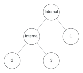
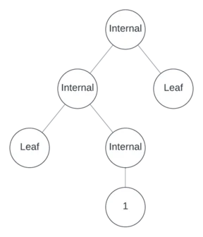
Typically, a CAS represents mathematical functions internally as binary-unary trees, also known as Motzkin trees: a network of nodes, each of which has 0, 1, or 2 children.
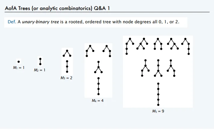
Examples of binary-unary trees1.
To translate functions to binary-unary trees, split the functions by their operators. Here’s an example:
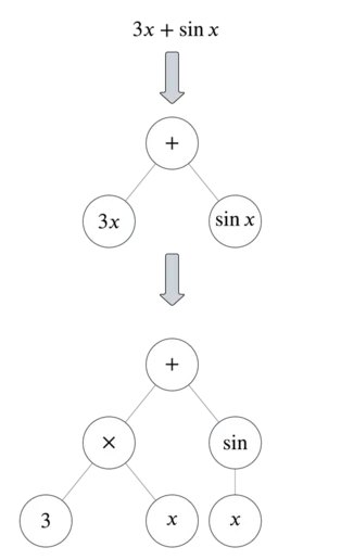
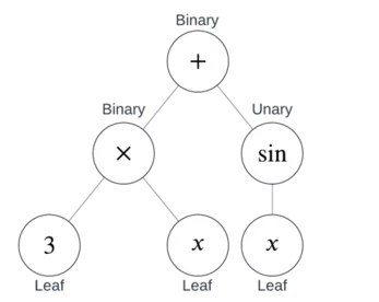
You can see from this example that there are three types of nodes:
- Leaves are nodes with no children, and correspond to constants and variables (like or ).
- Unary Nodes have one child, and correspond to unary operators (like or ).
- Binary Nodes have two children, and correspond to binary operators (like or ).
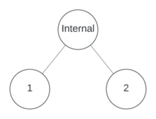
Together, binary and unary nodes are also known as Internal Nodes. In other words, an internal node is a node that’s not a leaf.
This is how a parser works in a CAS or graphing calculator.
Generating trees
This tree representation of functions makes it certain that a function is syntactically correct. To generate a function, generate a random binary-unary tree, and populate the nodes. Even this, though, is a non-trivial problem. Generating binary-unary trees efficiently is both well-studied2 and a topic of current research3. Since the trees I wanted to generate aren’t large, I opted for the simple algorithm presented by Lample and Charton.
The algorithm works by generating unassigned or “empty” nodes, and then “filling” them by deciding if they’re leaves, unary, or binary. First, decide how many internal nodes should be in the tree. In this case, suppose there should be three internal nodes.
Start with an empty node.

Since there’s only one node, it can’t be a leaf, so it will either be binary or unary. Suppose it’s binary.
Now that there are two empty nodes, decide the location of the next internal node. In this case, either the left node is an internal node, or it’s a leaf and the right node is internal. Note that to generate all possible trees with equal probability, this shouldn’t be a 50/50 choice! There exist more possible trees where the left node is internal than trees where it’s a leaf! I’ll get back to how calculating the sampling probability shortly.
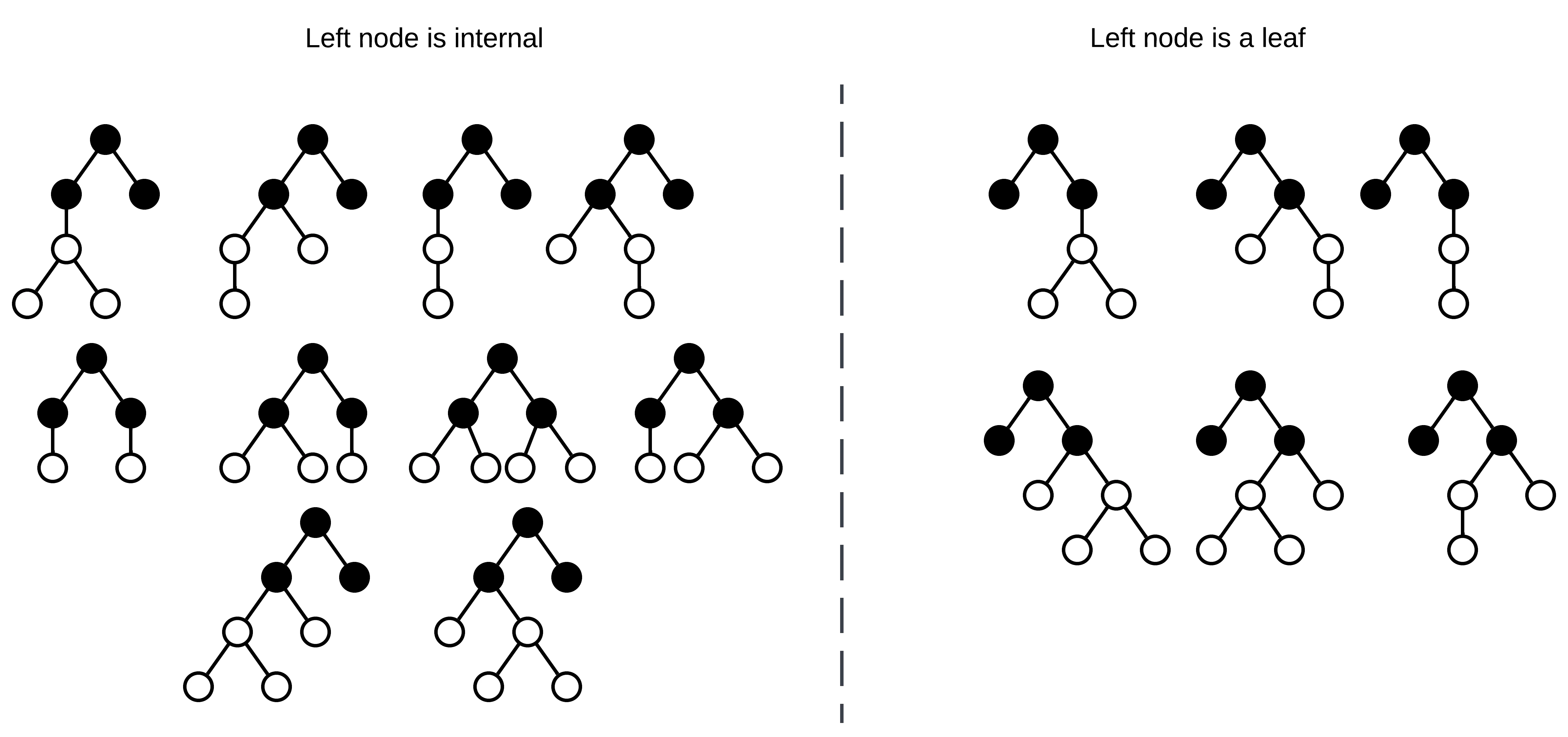
All possible binary-unary trees with three internal nodes.
Suppose the left node is internal, and further suppose that it’s binary. Now there are three empty nodes.
One more internal node remains to assign. Suppose it’s unary and in position 3, making the other positions leaves.
Now populate the tree with operators, variables, and numbers.
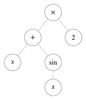
This tree represents .
Sampling with equal probability
When making the random decisions required to generate trees, all options can’t have equal probability, or the results will be unfair. Lample and Charton remark on this in the paper:
Naive algorithms (such as… techniques using fixed probabilities for nodes to be leaves, unary, or binary) tend to favor deep trees over broad trees, or left-leaning over right-leaning trees.
Each step, the random decisions reduce to a single choice. Given remaining internal nodes and empty nodes, assign the first nodes as leaves, and assign the next node as either a unary or binary node. The paper summarizes the probability of each option as:
is the probability that the next internal node is in position and has arity4 .
To calculate this probability, count all the possible trees before and after the choice. Assigning an internal node leaves remaining. If the node is unary, empty nodes become leaves, the unary node consumes another, but it creates a new one as its child, so the remaining empty nodes are .
A binary node is the same, but it has two children, leaving empty nodes.
To save space, use the notation:
Calculating this number recursively is possible with the following three insights:
-
If there are no more internal nodes to assign, only one tree is possible (the one you already have), so for all .
-
If there are no empty nodes, generating trees with any remaining internal nodes is impossible, so for all .
-
For and , there are three possibilities for the first node:
a. It’s a leaf, leaving empty nodes and internal nodes.
b. It’s a unary node, leaving empty nodes (one consumed and one produced) and internal nodes.
c. It’s a binary node, leaving empty nodes (one consumed and two produced) and internal nodes.
Restating insight 3:
Together, these form a recursive expression for . You can even calculate these values in Excel, if you want! Here’s a table of the first 10 values:
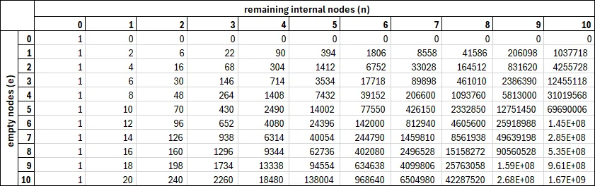
A table of the first 10 values of .

How the addition works.
To prevent this calculation taking up too much time, I memoized the function by caching its results (this combo, recursion and memoization, is also known as Dynamic Programming).
Now, with a way to calculate , define:
And:
Implementing in Python
Here’s a link to the Python module where I did this. I used Sympy, a Python CAS, to simplify the functions. To handle memoization, I used the functools @cache decorator.
Calculating integrals efficiently
Now that I had a big list of random functions, I needed to integrate them symbolically and save them for use in the training set. I decided on a SQLite table with the following three columns:
- Integrand: The function the program integrates.
- Integral: Either the result of integration, or
NULLif the integration wasn’t successful. - Success: True if integration succeeded, false otherwise.
To do the actual integration, I used Sympy again. Sympy is special—a free and open source computer algebra library written in pure Python. The following block of code can integrate lots of complicated functions!
import sympy as sp

def integrate_function(f: str) -> str:
    integral = sp.integrate(f, sp.symbols('x'))
    return str(integral)
Sympy does have some weaknesses, though. Python isn’t the fastest language (though it’s getting better!), so integrating with Sympy can be slow. Integration also hangs sometimes (which happens in basically any CAS).
To solve the performance issue, I wanted to perform integrations in parallel. To solve the hanging issue, I wanted integration to time out (something also done by the authors of the paper).
Python parallelism
Implementing parallelism in Python is tricky, because of the Global Interpreter Lock (GIL). The GIL exists because the Python interpreter isn’t fully thread-safe. Essentially it means that only one thread can access Python objects at one time. Opinions vary about the GIL, but PEP 703 says it best:
The GIL is a major obstacle to concurrency.
Because of this, Python has three main built-in approaches to concurrency. Two simulate parallelism, and one actually achieves it at a cost. When writing parallel Python code, understanding the differences between these approaches can help you understand what will actually speed your code up.
threadingis a module which makes many threads run tasks concurrently within the same interpreter. If code is I/O-bound (that is, it spends most of its time waiting for external events, like networking or APIs to other code), threading is well-suited, since threads won’t often try to access the same objects at once. If the long-running tasks involve manipulating Python objects or are CPU-bound, though, the GIL will prevent them from running simultaneously.asynciois a module for simulated concurrency on the same thread. Tasks run in an event loop, and when one task is waiting for network or disk operations, the interpreter switches to another task and works on it. Again, this is good for I/O-bound code (it’s great for web servers). It also is simpler than multithreading and more intuitive for people with asynchronous experience in other languages (like JavaScript). A common cliche is that you should “use asyncio when you can, and use threading when you must.” Asyncio has a similar limitation to threading: if one task is executing Python code it will block the event loop.multiprocessingis a different approach where processes spawn their own Python interpreters. True concurrency is possible because each process has its own GIL. Processes typically run on separate CPU cores, so hardware limits their number, and sharing state between processes is tricky.
In this case, the long-running tasks were all happening in Sympy, a pure Python program, and had no I/O component. This led me to believe that threading or asyncio would not make the program faster, but multiprocessing could. My desktop computer has 16 cores, so in theory I could speed the program up 16 times! To run the processes, I used concurrent.futures, which provides some high-level tools to run processes without needing to worry too much about cleanup. Here’s a basic sketch of how to do this:
def integrate_functions_parallel(functions: list[str]) -> list[str]:
    with ProcessPoolExecutor() as executor:
        results = list(
            executor.map(
                integrate_function,
                functions,
            )
        )
        return results
Time’s up
This solves the parallelism issue, but I still wanted timeouts. If a function takes a long time to integrate, it can clog up the whole process! Without timeouts, I worried that each process would waste most of its time on slow integrals which would never compute.
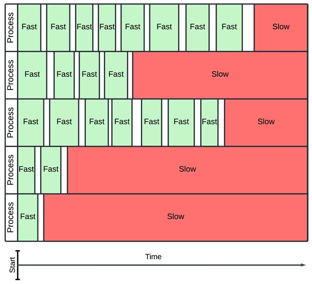
In this example, slow integrals dominate over fast ones, even though there are many more fast ones.
I chose to make processes time out with the wrapt timeout decorator. The timeout would raise an exception if any process took longer than a specified time. If this happened, I would catch the exception and count the integration as failed.
@timeout(INTEGRATION_TIMEOUT)
def integrate(f: str) -> str:
    integral = sp.integrate(f, sp.symbols(INTEGRATION_VARIABLE_NAME))
    if integral.has(sp.Integral):
        raise IncompleteIntegralException(
            f"Could not fully integrate {f}"
        )
    return str(integral)

def integrate_function_with_timeout(f: str, timeout: int) -> tuple:
    start_time = time()
    try:
        integral = integrate(f)
        return (f, integral, True)
    # Incomplete integration can raise a lot of different exceptions,
    # so I used the general catch here.
    except Exception as e:
        return (f, None, False)
Pesky processes
When I ran these functions, though, performance barely got faster. New processes weren’t getting picked up. I profiled the code with Scalene to figure out what was going on. Scalene could only account for about 30% of the execution time!
After some debugging, I realized that the timeout was elapsing and raising the exception, but not killing the integration process. The process was continuing to run in the background and consume resources. Soon, every CPU core would hang on these long-running processes, lowering the completion rate to almost zero.
To fix this, I had to manipulate the processes at a lower level—with the multiprocessing module instead of concurrent.futures. I used a multiprocessing.Queue object to hold the return value, and used the timeout parameter to return a process early if it timed out. To see if the process was still running, I would check is_alive, and terminate it if so.
def integrate_function(f: str, return_queue: multiprocessing.Queue) -> tuple:
    try:
        integral = sp.integrate(f, sp.symbols(INTEGRATION_VARIABLE_NAME))
        if integral.has(sp.Integral):
            raise IncompleteIntegralException(
                f"Could not fully integrate {f}"
            )
        return_queue.put((f, str(integral), True))
    except Exception as e:
        return_queue.put((f, None, False))


def integrate_function_with_timeout(f: str) -> tuple:
    return_queue = multiprocessing.Queue()
    process = multiprocessing.Process(
        target=integrate_function, args=(f, return_queue)
    )
    process.start()
    process.join(timeout=INTEGRATION_TIMEOUT)
    if process.is_alive():
        process.terminate()
        process.join()
        return (f, None, False)
    return return_queue.get()
Multi-computer parallelism
Running the program overnight, I generated about 12000 integrals. This was pretty good, but it paled in comparison to Lample and Charton’s 100 million. I wanted to run the code on more computers to speed it up.
Temporal
I learned how to use Temporal at work, and thought it would be perfect for this. Temporal is a runtime for durable, distributed function executions. Temporal provides tooling for retries, observability, debugging, testing, scheduling, and many other things.
It works by running a server (the Temporal Service) on one computer, which schedules and assigns tasks to Temporal Workers on many computers, which actually do the work. The server manages shared state between workers, and gives them instructions to do things. A user can add and remove workers at will, and all communication between workers and the server occurs over a network. Temporal is open source, and you can self-host or deploy on their cloud (which is how they make money5).

Temporal development network topology, from the Temporal docs.
To make my code run on temporal workers, I needed to separate it into workflows and activities that would run on the workers. An activity is a function which is failure-prone: in my case, integration and function generation. A workflow is a function which sequences and orchestrates activities. Workflows shouldn’t be prone to internal failures themselves, but they should be able to handle failing activities. Making the changes to my integration code was pretty easy; all I needed to do was add the activity.defn decorator.
@activity.defn
def integrate_function_with_timeout(f: str) -> tuple:
    # exact same code
I wrote a workflow class which would generate a batch of functions and then try to integrate them all. Workflow code is asynchronous, so I used asyncio.gather run all activities. Setting timeouts is mandatory, but I set them so that the functions’ internal timeouts would kill the processes first. At the end of the workflow, I used workflow.continue_as_new to start another, identical one, so that the integration process would run forever.
@workflow.defn
class GenerateAndIntegrateFunctionsWF:
    @workflow.run
    async def run(self, params: GenerateAndIntegrateFunctionsParams):
        functions = await asyncio.gather(
            *(
                workflow.execute_activity(
                    generate_function_with_timeout,
                    params.function_complexity,
                    start_to_close_timeout=timedelta(
                        seconds=GENERATION_TIMEOUT + 1
                    ),
                )
                for _ in range(params.batch_size)
            )
        )
        results = await asyncio.gather(
            *(
                workflow.execute_activity(
                    integrate_function_with_timeout,
                    f,
                    start_to_close_timeout=timedelta(
                        seconds=INTEGRATION_TIMEOUT + 1
                    ),
                )
                for f in functions
                if f is not None
            )
        )
        workflow.logger.debug(f"Results: {results}")
        await workflow.execute_activity(
            write_training_data,
            results,
            start_to_close_timeout=timedelta(seconds=10),
        )
        workflow.continue_as_new(params)
Since the activities were synchronous, running them in the asynchronous worker code required an activity_executor, and since they were running on separate processes, I needed a shared_state_manager to transfer information between them. I also had to register my workflows and activities on each worker.
async def main():
    client = await Client.connect(f"{TEMPORAL_SERVER}:{TEMPORAL_PORT}")

    worker = Worker(
        client=client,
        task_queue="default",
        workflows=[GenerateAndIntegrateFunctionsWF],
        activities=[
            generate_function_with_timeout,
            integrate_function_with_timeout,
            write_training_data,
        ],
        activity_executor=ProcessPoolExecutor(max_workers=MAX_WORKERS),
        shared_state_manager=SharedStateManager.create_from_multiprocessing(
            multiprocessing.Manager()
        ),
        max_concurrent_activities=MAX_WORKERS,
    )
    await worker.run()
The cluster
I ran the database and Temporal Service on my Raspberry Pi, which I’ve named Shasta after the famous mountain. I ran workers on Shasta, my desktop computer, my laptop, and my wife’s MacBook.
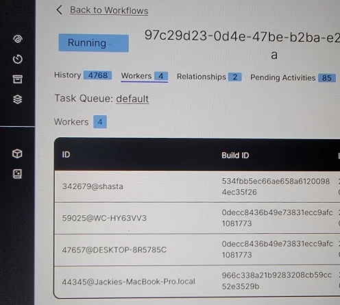
All four workers registered in the Temporal UI.
I switched from SQLite to Postgres in docker so that all workers could access the database. To enable access over my network, I had to change some ufw (firewall) settings. While I was doing that I closed port 22, disabling SSH. To re-enable it, I needed to actually plug a keyboard and mouse into the Raspberry Pi, something I’d avoided so far. Oh well.
While only one worker would run on each computer, each worker would run a process on each CPU. This meant I could run 44 concurrent processes!
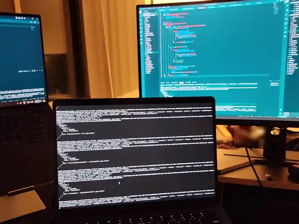
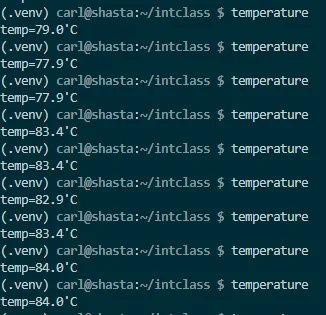
The cluster in action6!
Eventually I decided to suspend the worker on Shasta. Running all 4 cores at 100% was too much for the passive cooling case I bought. Maybe someday I’ll invest in a fan.
A little toasty.
This setup generated functions at about three times the speed, enough to generate a pretty big dataset.
Making the machine learn
I didn’t do anything groundbreaking here, but I’ll summarize:
- I fine-tuned MathBERT using this guide.
- I did the training on my desktop, running PyTorch with CUDA on a 4080.
- I trained the model for 3 epochs with a learning rate of , but stopped early on the first signs of overfitting.
- Accuracy on the validation set was about 95%.
- My code is here, feel free to check it out!
What I learned
This was a fun project! Even though it wasn’t for work, it felt like “real engineering.” Dealing with unreliable and hanging processes was fun, and challenged my assumptions about what happens when a process raises an exception. While I do some parallel and asynchronous computing at work, managing state between processes was pretty new to me. The cluster concept—having one computer run processes on another—felt magical. I’ve done this in cloud environments, but it feels different watching it happen in real life.
I’ve addressed a lot of complicated topics in this article, and it’s possible I’ve made a mistake! I’m new at a lot of this, but I don’t want to shy away from complex topics because of FOLD. If you think I should clear something up, you’re probably right! Send me an email.
References and footnotes
-
Sedgewick and Flajolet. An Introduction to the Analysis of Algorithms. (2013). Course Notes Chapter 5. ↩
-
Alonso. Uniform generation of a Motzkin word. (1994). Theoretical Computer Science. 134-2: 529-536. ↩
-
Lescanne. Holonomic equations and efficient random generation of binary trees. (2024). ArXiv: 2205.11982. ↩
-
Here “arity” is the same thing as node degree; a unary node has arity 1, and a binary node has arity 2. More on this concept. ↩
-
I’m not affiliated with Temporal, and I don’t care if you use it. I do have a pretty sweet pair of Temporal socks, though. ↩
-
I censored Jackie’s foot in the background, if you’re wondering about the mosaic. ↩